Most atmospheric science researchers use back-trajectory analysis in qualitative sense to explain source of a pollutant. And as pointed out by the questioner, it is not possible to associate trajectories calculated at a particular time to the measurement that is average of say several hours.
However, quantitative analysis of observed concentration with back-trajectories is possible and is used to identify emission sources and their strength.
For the quantitative analysis, a large number of back-trajectories are simulated (of the order of 100000) from the place of measurement, however each trajectory is initiated with slightly different initial condition.
Let me explain with an example. Suppose PM2.5 concentration was measured on a certain date as 24 hour average at location given by co-ordinates x, y and z. Assuming that air was well mix in region surrounding x, y and z given by x-dx to x + dx, y-dy to y+dy and z-dy to z + dy, backtrajectories will be simulated, each with slight different x,y and z but within volume given by 2dx*2dy*2dz. Also, the number of trajectories simulated will be equally distributed in the volume and time period (24 hours in this example) to which observation represents. The simulation will result in distribution of trajectory with some grid-boxes visited by several trajectories whereas others may have no trajectory or very few trajectories. Emissions in the grid-boxes which are more frequently visited, have more potential to contribute to observed concentration. In other words, the concentration being measured at x, y, z will be proportional to sum of amount of time spent by each trajectories multiplied by emission flux in that grid box.
More detailed description of backtrajectory analysis and its application to related to observed quantity are available in following articles.
Gadhavi et al., 2015, Evaluation of black carbon inventories using a Lagrangian dispersion model - a case study over Southern India, Atmos Chem Phys, vol. 15, 1447-1461, doi: 10.5194/acp-15-1447-2015.
Seibert and Frank, 2004, Source-receptor matrix calculation with a Lagragian particle dispersion model in backward mode, Atmos. Chem. Phys., vol. 4, 51-63, doi:10.5194/acp-4-51-2004
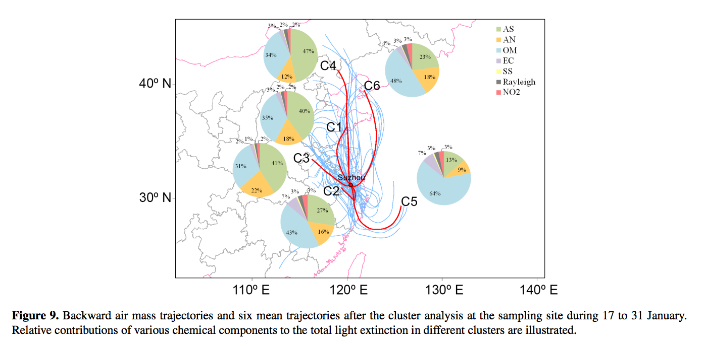
 In this figure from Characteristics of aerosol pollution during heavy haze events in
Suzhou, China, the trajectories are clustered into several groups. The different fractions of chemicals (e.g. organic matter, sulfate) in each group shows the impact of different regions.