The time-averaged material transport by water waves is quantified by Stokes drift, which is the residual Lagrangian drift due to sub-surface orbits not being closed:
$$
u_{St} = \dfrac{\omega k^2 a \cosh[2k(z+d)]}{2\sinh(kd)^2}
$$
where $\omega$ is the angular frequency, $k$ is the wavenumber, $a$ is the wave amplitude, $d$ is mean water depth, and $z$ is the displacement from water surface, positive upward.
Because the cave is closed, there is build-up of water in the cave which results in pressure gradient-induced Eulerian backflow which opposes the Stokes drift. This backflow is barotropic in nature and equals:
$$
u_E = -\dfrac{1}{d}\int_{-d}^{0}u_{St}(z)dz
$$
The transport velocity is the sum of mean Eulerian velocity and Stokes drift:
$$
u_L = u_E + u_{St}
$$
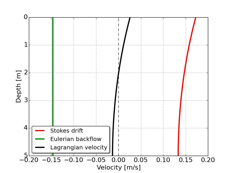
For the case of $T = 12\ s$, $a = 1\ m$, and $d = 5\ m$, the resulting transport looks like this:

Because the Stokes drift is not uniform in the vertical but compensating Eulerian backflow is, the resulting transport is into the cave in the upper 2 m, and out of the cave below that depth.
Assumptions made:
- Inviscid ($\mu\nabla^2\mathbf{u}=0$), irrotational ($\nabla \times \mathbf{u} = 0$), and incompressible ($\nabla\cdot \mathbf{u}=0$) flow.
- Small amplitude for the linear wave theory to hold.
- All wave energy is dissipated at the cave wall (no reflection). If there is some reflection of waves out of the cave, then the Stokes drift and the corresponding Eulerian backflow would be reduced in magnitude, but the answer for the net transport would be qualitatively the same.
- Shallow water dispersion relationship ($\omega^2 = gk^2d$).
And here is the Python code:
import numpy as np
import matplotlib.pyplot as plt

T = 12. # wave period [s]
d = 5.  # mean water depth [m]
a = 1.  # wave amplitude [m]
g = 9.8 # gravitational acceleration [m/s]

omega = 2*np.pi/T # angular frequency [rad/s]
k = np.sqrt(omega**2/(g*d)) # wavenumber [rad/m]

z = np.linspace(0,-d,501.) # depth array [m]
dz = -np.gradient(z) # depth increment [m]

# Stokes drift in arbitrary depth
ust = 0.5*omega*k*a**2*np.cosh(2*k*(z+d))/np.sinh(k*d)**2

# Eulerian backflow is the vertical integral of Stokes drift
ue = -np.ones(z.size)*np.sum(ust*dz)/d

fig = plt.figure(figsize=(8,6))
ax = fig.add_subplot(111,xlim=(-0.2,0.2),ylim=(5,0))
ax.tick_params(axis='both',which='major',labelsize=16)
plt.plot(ust,-z,'r-',lw=3,label='Stokes drift')
plt.plot(ue,-z,'g-',lw=3,label='Eulerian backflow')
plt.plot(ust+ue,-z,'k-',lw=3,label='Lagrangian velocity')
plt.plot([0,0],[5,0],'k--')
plt.legend(loc='lower left',shadow=True,fancybox=True)
plt.grid(True)
plt.xlabel('Velocity [m/s]',fontsize=16)
plt.ylabel('Depth [m]',fontsize=16)
plt.savefig('transport.png',dpi=100)
plt.close(fig)
