Staggered Grid finite difference implementation for modelling the elastic wave equation in 2D?

Question

I am attempting to implement FD in 2D with a staggered grid scheme as per (Virieux 1986). I am having difficulties going from the numerical analysis formulas to the code for this particular scheme. As I have not seen any concrete examples for staggered grid FD.

I would love to see an example. If anyone could link a book, paper or a webpage, It would be immensly appreciated.

Cheers,

Answer 1

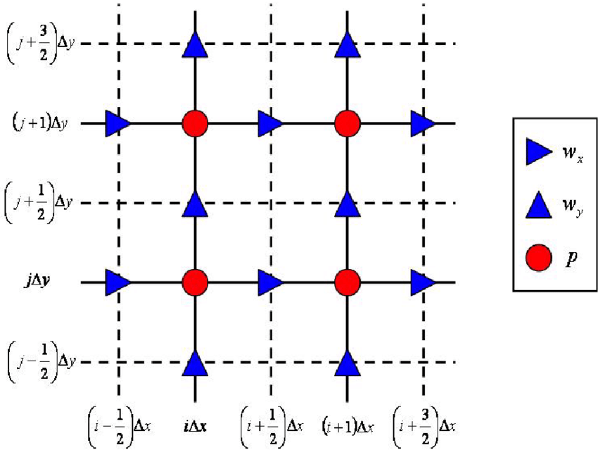
Here is a simple MATLAB script for a simple FD implementation (2nd order accurate in space and time) for the acoustic wave equation, which is identical to Virieux (1986) under the assumption of $\mu=0$ and $\sigma_{xx}=\sigma_{zz}=-p$ for pressure $p$. Let me know if that helps or not, and maybe we can update the answer from there.

The main confusion in staggered grid modeling is that you have multiple grids (here, e.g., pressure $p$ and the horizontal and vertical particle velocities $v_x$ and $v_z$), and the computer implementation only allows you to index them at full integers p[1], p[2], vx[1], ..., but in practice they may be offset, i.e., the location of p[1] is not the same location as vx[1], they are actually offset by $\Delta x/2$, just indexed by the same integer.

Figure copied from https://www.researchgate.net/figure/Spatially-staggered-finite-difference-grid-for-solution-of-acoustic-wave-propagation_fig1_235037633 . The code is my own.

%% Setting up the spatial & temporal model
% --- The true dimensions (in meters)
lx = 1200;
ly = 1200;

% --- The true total run-time (in seconds)
lt = 5;

% --- The true medium parameters (m/s and kg/m3)
vp  = 2000;
rho = 1500;

% --- The finite-difference parameters
dx = 2;
dy = dx;
dt = 0.5e-3;

% --- The associated discrete grid in space and time
nx = floor(lx/dx);
ny = floor(ly/dy);
nt = floor(lt/dt);
x = [0:nx-1]*dx;
y = [0:ny-1]*dy;
t = [0:nt-1]*dt;

% --- Source-time wavelet (supply central frequency fc, in Hertz)
ricker = @(fm,t) (1-2*pi^2*fm^2*t.^2) .* exp(-pi^2*fm^2.*t.^2);
fc = 20;
fs = ricker(fc, t-0.1 ); % Time-delayed Ricker wavelet (plot, if desired!)

% --- Source location (positioned at 400, 600)
[~,sidx] = min(abs(x - 400));
[~,sidy] = min(abs(x - 600));

%% The computational loop
% Initialize fields
p = zeros(nx+1,ny+1);
vx = zeros(nx+1,ny+1);
vy = zeros(nx+1,ny+1);

% Stencil update locations
X = 1:nx;
Y = 1:ny;

figure(1);
for a = 1:nt
    % (1) Inject source funtion
    p(sidx,sidy) = p(sidx,sidy) + dt*fs(a);
    
    % (2) Update p
    p(X+1,Y+1) = p(X+1,Y+1) - (dt*rho*vp^2)*((vx(X+1,Y) - vx(X,Y))/dx ...
                                            +(vy(X,Y+1) - vy(X,Y))/dy );
    
    % (3a) Update ux
    vx(X,Y) = vx(X,Y) - (dt/rho)*(p(X+1,Y+1) - p(X,Y+1))/dx;
    
    % (3b) Update uy
    vy(X,Y) = vy(X,Y) - (dt/rho)*(p(X+1,Y+1) - p(X+1,Y))/dy;
    
    % Display every 10th computation
    if (mod(a,10)==0)
        imagesc(x,y,p');
        axis equal;
        title(['Timestep = ', num2str(a), 'dt']);
        xlabel('x [m]');
        ylabel('y [m]');
        drawnow
    end
end