Simple Climate Models that Predict Climate Change

Question

I have a physics/maths background, and to me the most convincing evidence of a scientific fact is often a very simple model that gives reasonable results. A simplified model, which you can fully understand, is often more convincing than the numerical output of a complex model.

So I'm looking for a simple climate model, which could be used to predict how increasing $\ce{CO_2}$ concentrations would lead to an increase in temperature. For instance, this model need not account for the specific geography of the earth: it might just consider the sun's radiation passing through an atmosphere and striking a flat, homogeneous surface with some constant absorptivity. Then we could just do an energy balance to find equilibrium temperature as a function of $\ce{CO_2}$ concentration.

If I could do a back-of-the-envelope calculation to see that doubling $\ce{CO_2}$ concentrations would be expected to increase the Earth's temperature by a few degrees (I expect nothing more than this order-of-magnitude evidence) then I think that would be convincing evidence that climate change is worth worrying about. You can argue with satellite data and complex models, but you can't argue with basic physics.

So far, the only source I've found that gives such a simplified model is Arrhenius himself, in his 1896 paper. I actually find his model quite convincing, and its prediction ($\sim5^oC$ increase from doubling $\ce{CO_2}$) gives a reasonable prediction too. However, his data on the absorptivity of the atmosphere was (rather quaintly) obtained by early measurements of the intensity of moonlight at different angles in the sky. While this is ingenious, I'm sure with modern technology we could get much better estimates.

So I'm basically looking for either a modernised version of Arrhenius' calculations, or alternatively another simple model which convincingly demonstrates that increasing $\ce{CO_2}$ has the power to alter the earth's temperature by as much as a few degrees.

Answer 1

It sounds like you are asking for a simple climate model that treats the globe as a homogeneous system. A Zero-dimensional energy balance model may be of interest (see this Penn State site ) which uses a starting point that is also basically described in this post: Temperature as a function of luminosity and greenhouse gas concentrations

If you solve for the temperature of the Earth using a blackbody approximation and thermal equilibrium (with an albedo of about 0.3), you are only taking into account the temperature of the Earth without a greenhouse effect (about 33 °C cooler than actual temperature). It is very difficult to calculate the influence of infrared radiative forcing components (e.g. oxygen and carbon dioxide) to an empty atmosphere, since there are many biogeochemical/physical feedbacks in the climate system which are nonlinear.

However, if you start with current temperature/concentrations, you can add terms that represent particular increases to the GHG concentrations. Those terms are constantly being refined by the scientific community and are summarized in this Wikipedia article about Radiative Forcing (see the link to climate sensitivity at the bottom of the page). This is a kind of "back of the envelope" modeling approach that most climate scientists use to discuss past and future influence of climate forcers, which can be very helpful when discussing the expected climate effects of various emissions/mitigation scenarios.

The Radiative Forcing article in Wikipedia says:

Radiative forcing can be used to estimate a subsequent change in equilibrium surface temperature (ΔTs) arising from that radiative forcing via the equation:

$$\Delta T_s =~ \lambda~\Delta F$$

where λ is the climate sensitivity, usually with units in K/(W/m²), and ΔF is the radiative forcing. A typical value of λ for CO₂ is 0.8 K/(W/m²), which gives a warming of 3K for a doubling of CO₂ [from pre-industrial times, assuming RF of CO₂ is ~ 3.7)].

It's important to note that most climate sensitivity parameters and radiative forcing values are derived with respect to some time period (e.g. 1750 - 2011) and GHG feedbacks are set for a particular climate regime. Revised radiative forcing and climate sensitivity parameters are needed to make calculations for other climate regimes.

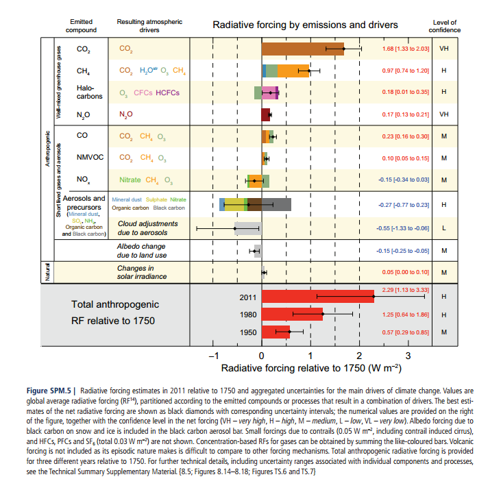
The IPCC AR5 figure of Radiative Forcing components attributes 1.65 W/m² to the actual increase in CO₂ concentrations from 1750 to 2011 (or ~1.3K in temperature rise, if lambda is 0.8).

The values of Radiative Forcing that IPCC provides are likely close enough for doing realistic scenario testing. However, something in an entirely different feedback regime would need very different parameters. For instance, halving the CO₂ in the atmosphere would have a much greater absolute effect on temperature than doubling it; temperature increases logarithmically as CO₂ concentrations increase. This is because strong CO₂ absorption bands are nearly saturated under present conditions, and increasing CO₂ from present conditions mainly affects the flanks of the absorption bands. However, water precipitates out of the system easily under low-temperature conditions, so CO₂ has a much greater forcing value in those types of climate regimes.

The most difficult problems with testing simple climate scenarios are related to the oceans and the biosphere, which could have countless effects on the average climate and GHG regime.

Answer 2

The Meteorological Institute of the University of Hamburg, Germany, provides and simple model called "Planet Simulator" (PlaSim).

The Planet Simulator is mainly made for educational purposes and runs on personal computers. However, it is also parallalized and can be run on HPC clusters. There exists an Documentation and the source code is said to be well commented. The whole source code is open source. The programming language is Fortran. One should be able to compile it with gfortran under Linux.

The Planet Simulator offers a GUI (after compiling successfully) to set up da model simulation and run it. There is code for postprocessing included. Thus, there is not need for additional postprocessing software. If you write out the output as netCDF, which is the quasi-standard output format of climate models, it might be practical to install ncview or Panoply because these are common netCDF viewers with which you can look directly into the output files.

Answer 3

Start with the Earth's radiative equilibrium temperature T_e:

S (1 - A) [T_e] = 4 _e²] e s Te⁴

where S is the Solar constant, A the planetary albedo, pi the circle constant (3.14159...), R_e the Earth's radius, e emissivity, s the Stefan-Boltzmann constant, and T_e the temperature we're looking for. Solving for T_e, [T_e] cancels, and S 1361.5 W m^-2, A 0.294, e 1 (always taken as 1 at the top of a planet's atmosphere) gives you Te = 255 K.

This is below freezing, since water freezes at 273 K, so obviously something else keeps the surface hotter--the greenhouse effect. Actual surface temperature Ts is now about 288 K. A simple (too simple) model is the Milne-Eddington approximation:

T_s = T_e(1 + 0.75 τ)^0.25

where tau is the atmosphere's long wave optical depth. The present value of this is about 1.84, which gives you T_s = 317 K, too high. This is because this approximation fails to account for surface cooling by convection and conduction.

The more greenhouse gases you have in the atmosphere, the higher τ gets, and the higher T_s goes. Many "semigray" approximations model partial τ ("partial" meaning for each gas) as a function of the gas's partial pressure, usually raised to some power. Add up the partials to get tau. It may help to know that at present, water vapor accounts for about 50% of τ, clouds 25%, carbon dioxide 20%, and minor gases (CH₄, O₃, N₂O, etc.) 5%.

I hope this is enough to get you started.