The unit mole / m² has dimensions count per area; the unit µg / m³ has dimensions mass per volume. To go from a quantity per area to a quantity per volume, you need to understand some properties of the instrument.
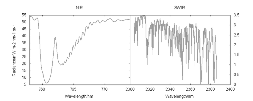
The spectrometer on Sentinel-5P is TROPOMI. TROPOMI is an imaging spectrometer, meaning it measures the spectrum of top-of-atmosphere electromagnetic radiation at various wavelengths. Such a spectrum (the "level 1 data") may look like this:

Source: Hu et al. (2016), DOI:10.5194/amt-2016-108, CC-BY 3.0
Original caption:
Simulated TROPOMI spectra in the NIR and SWIR channels for a scenario from the global ensemble,
For most users, these spectra do not readily show what they are actually interested in. However, from these spectra it is possible to calculate the atmospheric composition of various trace gases, because each gas has its own unique spectral signature. How this works is too complicated to explain in a Stack Exchange answer, but is covered in text books and university courses.
For a down-looking instrument like TROPOMI, it is difficult to resolve vertical information. For some species (some trace gases) we may have a rough idea whether the quantities calculated are close to the surface or close to the top of the atmosphere, for others we really only have a clue about the total column amount (meaning the total amount between the surface and the satellite). Therefore, when a data product reports a column integrated amount, it is not possible to assign this to a specific height.
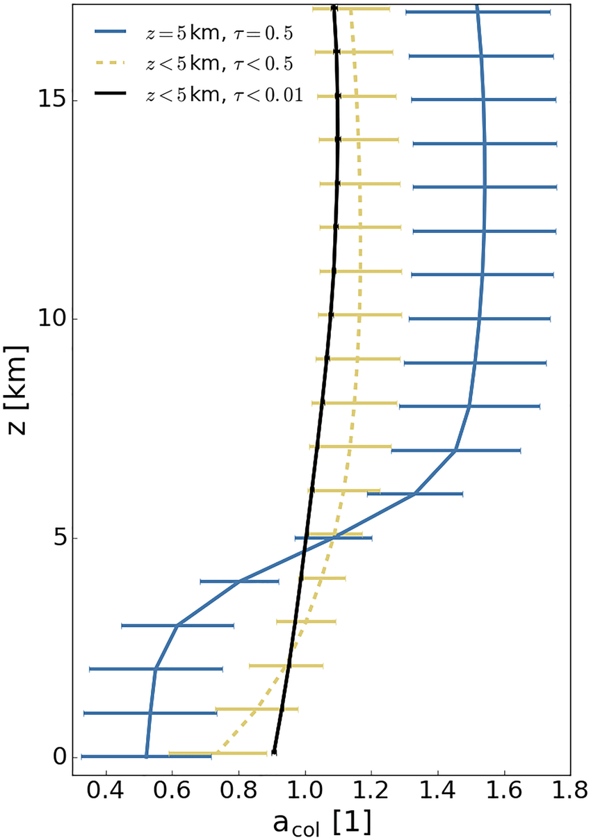
However, a retrieval may be more sensitive for some heights than for others. Maybe it mostly sees the top part of the column, maybe mostly the bottom part. One way to express this is by the averaging kernel. The averaging kernel tells you to what height the total column measurement is most sensitive:

Source: Borsdorff et. al (2018), DOI:10.5194/amt-11-5507-2018, CC-BY 4.0
Original caption:
TROPOMI CO total column averaging kernels for 10 November 2017. The global average is shown for three different categories of cloudiness strict cloud clearing (black), clear-sky equivalent (yellow), and high optical thick clouds (blue). The standard deviation is indicated as error bars.
What does this mean? Firstly, the averaging kernel is situation dependent. Maybe that's why you've been told you need the height of the inversion layer, but more likely people may use the height of the inversion layer to model where certain species are likely to be located, using a model that simulates atmospheric chemistry and dynamics. The figure shown here shows global averages for those averaging kernels for a single day (at least that what it claims; more likely it shows the average of all measurements, which is not strictly the same, as the instrument samples some places more than others). Secondly, it's very broad. The black line shows the case for clear-sky. The averaging kernel is rather flat, meaning that CO at various heights contributes pretty much equally to the total column amount. The blue line shows more sensitivity to upper parts of the atmosphere, but that's because the lower part is obscured by clouds.
In this case, there is no vertical height to convert from mole/m² to µg/m³. I suppose you could estimate the mass of a column of atmosphere, but it's more conventional to report in mole/m², such as your source does. Or you could use an atmospheric chemistry model that estimates what a likely vertical distribution looks like, based on various characteristics. I'm not an atmospheric chemist so I can't say a lot about how well that works.
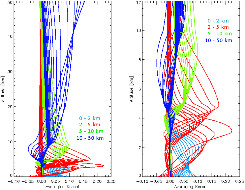
Some averaging kernels look more narrow (NB: not TROPOMI). I think this one is about simulated aerosol retrievals with different channels:

Source: Colosimo et. al (2015), DOI:10.5194/amtd-8-11853-2015, CC-BY 3.0
Original caption:
Example of averaging kernel vs. altitude. The simulation refers to a convolved spectrum of spectral resolution ∆ν = 0.01 cm −1 and FWHM = 0.05 cm −1 with a solar zenith angle SZA = 45 • and an instrument viewing angle of 30 • off-nadir. The AK are color coded for different altitude ranges. On the right, a zoom between 0 and 12 km is shown.
In this case, some vertically resolved information is available.
To truly get vertically resolved information, you want to use a limb sounder. Instead of looking down, a limb sounder looks at the horizon, scanning up and down. Each measurement only sees a narrow vertical section of the atmosphere. However, it has a poor horizontal resolution and worse temporal sampling. In the special case of solar occultation, the signal to noise ratio gets very high, but any given location only has measurements about twice a year. Comparing the three is possible. From personal experience, I can tell you that this is a challenge for any scientist :)
Followup question
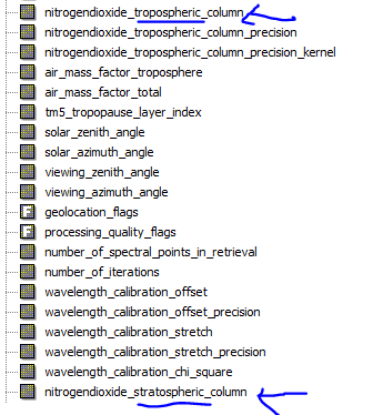
The Sentinel product gives you different layers, as you can see in the image, the NO2 gives a layer of tropospheric data and another of stratospheric data... by making this separation, shouldn't they be assuming a limit to the height of the column in which the data is separated by layers?
Yes, they should. They have different channels that are sensitive to different heights, but this sensitivity is still rather broad. For example, maybe they have a channel that's sensitive to 0-8 km, 2-10 km, 4-14 km, 6-16 km, 8-20 km, 10-30 km, then use a numerical method to estimate the partial column for 0-12 km and 12-30 km. If I see such a claim, I would look closely at the papers describing the retrieval method to see how exactly they calculated what they call tropospheric and stratospheric data. I haven't read those papers in case of TROPOMI, but as a downlooking spectrometer, it's not going to be a sharp cutoff. Maybe the user guide has some information that can help with the vertical attribution?
 I understand that the height of the limit of these can vary, but I would like to arrive at an approximate average value.